05. 线性回归的扩展

来源：原始 Jupyter Notebook。内容已转换为网页阅读格式；下载原文件。

在现实生活中，纯粹的线性模型是很难遇到的，我们不妨再来看看下面的数据集：

x	y
40	216
50	399
60	496
70	507
80	432
90	271

如果我们按照线性回归的解法，也能得到解，如下所示：

import numpy as np

X = np.matrix([
    [1, 1, 1, 1, 1, 1], 
    [40, 50, 60, 70, 80, 90]]).T
Y = np.matrix([216, 399, 496, 507, 432, 271]).T

a = (X.T * X).I * X.T * Y
print("a = {0}".format(a))

运行结果

a = [[315.33333333]
 [  1.1       ]]

得到一元线性回归：

y = 1.1x + 315.33

我们画出回归线和散点数据：

import numpy as np
import matplotlib.pyplot as plt

plt.xlim(30, 100)
plt.ylim(100, 600)

X = np.array([40, 50, 60, 70, 80, 90])
Y = np.array([216, 399, 496, 507, 432, 271])
plt.scatter(X, Y)

x = np.linspace(30, 100)
y = 1.1*x+315.33
plt.plot(x, y)

plt.show()

运行结果

Notebook 运行结果

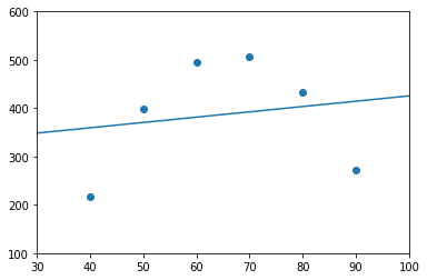
从图中很容易看出，线性回归对数据的拟合度不是很高，很显然散点的分布不是直线，而是一个二次曲线。我们知道二次曲线通常可以写成这样：

y = a_0 + a_1x + a_2x^2

到现在为止，我们一直在处理线性回归问题，那么对于这种不是线性的情况，该如何求解呢？首先，看到上面这个式子，我们不由得联想到了我们之前遇到的二元线性回归：

y = a_0 + a_1x_1 + a_2x_2

二元线性回归问题处理的是两个自变量，但是我们这里只有一个自变量，怎么办呢？答案是：自己造一个出来。

x	$x^2$	y
40	1600	216
50	2500	399
60	3600	496
70	4900	507
80	6400	432
90	8100	271

我们引入一个新变量 $x^2$ ，令： $x_1 = x, x_2 = x^2$ ，这样我们就可以像处理线性回归问题一样处理非线性回归问题了。

import numpy as np

X = np.matrix([
    [1, 1, 1, 1, 1, 1], 
    [40, 50, 60, 70, 80, 90],
    [1600, 2500, 3600, 4900, 6400, 8100]]).T
Y = np.matrix([216, 399, 496, 507, 432, 271]).T

a = (X.T * X).I * X.T * Y
print("a = {0}".format(a))

运行结果

a = [[-1376.  ]
 [   57.  ]
 [   -0.43]]

得到回归问题的解：

\begin{align} y &= 57x_1 - 0.43x_2 - 1376 \\ &= 57x - 0.43x^2 - 1376 \end{align}

画出二次曲线图，拟合度非常高：

import numpy as np
import matplotlib.pyplot as plt

plt.xlim(30, 100)
plt.ylim(100, 600)

X = np.array([40, 50, 60, 70, 80, 90])
Y = np.array([216, 399, 496, 507, 432, 271])
plt.scatter(X, Y)

x = np.linspace(30, 100)
y = 57*x - 0.43*x*x - 1376
plt.plot(x, y)

plt.show()

运行结果

Notebook 运行结果

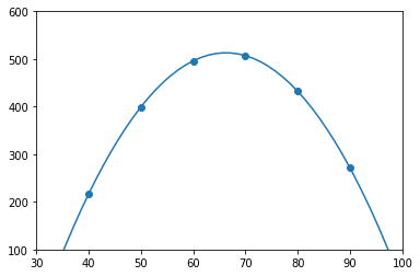
一元二次回归的求解可以转换为二元线性回归的求解。依葫芦画瓢，当我们遇到一元三次，一元四次，或一元 N 次曲线时，也可以将自变量 $x$ 扩充为 $x^3$ ， $x^4$ 或 $x^N$ ，从而转换为 N 元线性回归的求解。如果自变量不止一个，譬如二元三次曲线，也可以使用同样的方法，只不过要注意自变量之间的组合。这被称为线性回归的扩展。

我们用数学语言来描述的更清晰一点。对于一元线性模型，我们记为：

y = ax + b

其中，a、b、x 都是标量，如果把 x 变成关于 x 的函数向量 $\phi(x)$ ，同时把参数 a 变成关于函数向量 $\phi(x)$ 的参数向量 $\bf{\theta}$ ，那么可以得到线性模型的一个扩展：

\begin{align} y &= \theta_1\phi_1(x) + \theta_2\phi_2(x) + ... + \theta_k\phi_k(x) \\ &= \sum_{i=1}^k\theta_i\phi_i(x) \\ &= \bf{\theta}^T\phi(x) \end{align}

这里我们把 $\phi(x)$ 叫做 基函数（basis function），当我们把 $\phi(x)$ 定义为：

\phi(x) = (1, x, x^2)^T

我们就得到了上面的一元二次回归模型，更一般的，当我们把 $\phi(x)$ 定义为多项式形式：

\phi(x) = (1, x, x_2, ..., x^{k-1})^T

我们就可以得到更通用的 多项式回归 模型，当我们把 $\phi(x)$ 定义为三角多项式形式：

\phi(x) = (1, \sin x, \cos x, \sin 2x, \cos 2x, ..., \sin mx, \cos mx)^T

我们就可以得到了 三角多项式回归 模型。像这样把本来是一维的模型扩展成多维模型，叫做升维。

基函数是构成函数空间的基础，就好像基向量是构成向量空间（线性空间）的基础一样，函数空间中的任何一个函数都可以表示成基函数的线性组合。在数值分析和近似理论中，基函数也被称为混合函数（blending function），常常用于插值（interpolation）。上面的多项式回归使用的基函数叫做多项式基，三角多项式回归使用的基函数叫做傅里叶基。此外，基函数还是核方法（Kernel method）和字典训练的基础。

但是这种扩展只能针对输入变量是一维的情况，对于多维的输入向量 $\bf{x}$ ，基函数该如何选取呢？对于这种情况，一般有两种扩展方法：一种是通过基函数相乘来得到扩展模型，这种模型称为 乘法模型，另一种是通过基函数相加得到扩展模型，这种模型称为 加法模型。假设 $\bf{x}$ 是一个 d 维向量 $(x_1, ... x_d)^T$ ，n 表示各维的参数个数，那么乘法模型可以记为：

y = \sum_{j_1=1}^{n} \dots \sum_{j_d=1}^{n} \theta_{j_1 \dots j_d} \phi_{j_1}(x_1) \dots \phi_{j_d}(x_d)

加法模型可以记为：

y = \sum_{i=1}^d \sum_{j=1}^n \theta_{i,j} \phi_{j}(x_i)

上面的公式看起来可能很复杂，不过我们可以通过一个简单的例子把上式展开来看看，假设维数 d = 2，也就是 $\bf{x} = (x_1, x_2)^T$ ，基函数为多项式形式并且 n = 3，也就是 $\phi(x) = (1, x, x^2, x^3)$ ，很容易得出乘法模型：

\begin{align} y &= \sum_{i=1}^3 \sum_{j=1}^3 \theta_{ij} \phi_i(x_1) \phi_j(x_2) \\ &= \sum_{i=1}^3 (\theta_{i1} \phi_i(x_1) \phi_1(x_2) + \theta_{i2} \phi_i(x_1) \phi_2(x_2) + \theta_{i3} \phi_i(x_1) \phi_3(x_2)) \\ &= \theta_{11} \phi_1(x_1) \phi_1(x_2) + \theta_{12} \phi_1(x_1) \phi_2(x_2) + \theta_{13} \phi_1(x_1) \phi_3(x_2) \\ &+ \theta_{21} \phi_2(x_1) \phi_1(x_2) + \theta_{22} \phi_2(x_1) \phi_2(x_2) + \theta_{23} \phi_2(x_1) \phi_3(x_2) \\ &+ \theta_{31} \phi_3(x_1) \phi_1(x_2) + \theta_{32} \phi_3(x_1) \phi_2(x_2) + \theta_{33} \phi_3(x_1) \phi_3(x_2) \\ &= \theta_{11} x_1 x_2 + \theta_{12} x_1 x_2^2 + \theta_{13} x_1 x_2^3 \\ &+ \theta_{21} x_1^2 x_2 + \theta_{22} x_1^2 x_2^2 + \theta_{23} x_1^2 x_2^3 \\ &+ \theta_{31} x_1^3 x_2 + \theta_{32} x_1^3 x_2^2 + \theta_{33} x_1^3 x_2^3 \end{align}

加法模型：

\begin{align} y &= \sum_{i=1}^2 \sum_{j=1}^3 \theta_{ij} \phi_j(x_i) \\ &= \sum_{i=1}^2 (\theta_{i1} \phi_1(x_i) + \theta_{i2} \phi_2(x_i) + \theta_{i3} \phi_3(x_i)) \\ &= \theta_{11} \phi_1(x_1) + \theta_{12} \phi_2(x_1) + \theta_{13} \phi_3(x_1) \\ &+ \theta_{21} \phi_1(x_2) + \theta_{22} \phi_2(x_2) + \theta_{33} \phi_3(x_3) \\ &= \theta_{11} x_1 + \theta_{12} x_1^2 + \theta_{13} x_1^3 \\ &+ \theta_{21} x_2 + \theta_{22} x_2^2 + \theta_{33} x_3^3 \end{align}

乘法模型是将基函数两两相乘，要回归的参数个数为 $b^d$ ，而加法模型只是将所有的基函数相加，所以要回归的参数个数为 $b \times d$ ，很显然，乘法模型的表现力要丰富的多，但是乘法模型的参数个数是呈指数级増长的，当输入参数的维度增加到 100 时，要回归的参数个数就增加到 $2^100$ 个，这个计算量是非常大的。这种随着维度的增加，计算量呈指数级増长的现象，通常称为 维数灾难 或 维数诅咒（curse of dimensionality）。

无论是上面介绍的一维情况下的多项式回归模型，还是多维情况下的乘法模型或加法模型，本质上都还是线性回归。

我们假设基函数 $\phi(x) = (\phi_1(x), \phi_2(x), \dots, \phi_b(x))$ ，于是有下面的 $n \times b$ 阶矩阵，被称为设计矩阵：

\[ \Phi = \left ( \begin{array}{ccc} \phi_1(x_1) & \phi_2(x_1) & \dots & \phi_b(x_1) \\ \vdots & \vdots & \vdots & \vdots \\ \phi_1(x_n) & \phi_2(x_n) & \dots & \phi_b(x_n) \end{array} \right ) \]

基于基函数的线性模型可以表示成：

f_{\theta}(x) = \Phi \theta

损失函数为：

J(\theta) = \frac{1}{2} \| \Phi \theta - y \|^2

和前面多元线性回归的求解一样，我们得到其最小二乘解为：

\hat{\theta} = (\Phi^T\Phi)^{-1}\Phi^T y = \Phi^{\dagger}y

使用这种方法我们可以对线性模型进行无限的扩展，譬如我们把设计矩阵 $\Phi$ 替换为下面的 核矩阵 $K$ ：

\[ K = \left ( \begin{array}{ccc} K(x_1, x_1) & K(x_1, x_2) & \dots & K(x_1, x_n) \\ \vdots & \vdots & \vdots & \vdots \\ K(x_n, x_1) & K(x_n, x_2) & \dots & K(x_n, x_n) \end{array} \right ) \]

我们就得到了 核模型：

f_{\theta}(x) = \sum_{i=1}^n \theta_i K(x, x_i)