06. Scikit Learn 中的 SVM

来源：原始 Jupyter Notebook。内容已转换为网页阅读格式；下载原文件。

这一节我们使用 sklearn 中提供的 SVM 方法来解决一个简单的二分类问题。sklearn 自带了一个鸢尾花的数据集，这个数据集是 Fisher 在 1936 年收集整理的，是一类多重变量分析的数据集，数据集共包含 150 条数据记录，分为 3 类，每类 50 个数据，每条数据包含 4 个属性。可通过花萼长度，花萼宽度，花瓣长度，花瓣宽度 4 个属性预测鸢尾花卉属于（Setosa，Versicolour，Virginica）三个种类中的哪一类。

由于我们想使用 SVM 解决二分类问题，所以这里我们只取鸢尾花的两种类型，每种类型只取两个特征：

import numpy as np
import matplotlib.pyplot as plt
from sklearn import datasets

iris = datasets.load_iris();

X = iris.data
y = iris.target

X = X[y < 2, :2]
y = y[y < 2]

plt.scatter(X[y == 0, 0], X[y == 0, 1], color='red')
plt.scatter(X[y == 1, 0], X[y == 1, 1], color='blue')
plt.show()

运行结果

Notebook 运行结果

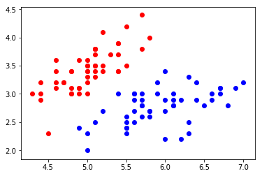
图中可以看出数据非常明显的分为两类。通过 sklearn 中提供的 LinearSVC 类，可以非常方便的训练出模型，这里的参数 C 取一个很大的数字，这样得到的接近于硬间隔支持向量机。我们输入两个测试数据：(6,2) 和 (4,3) 得到的结果正好是 1 和 0。

from sklearn.svm import LinearSVC

svc = LinearSVC(C=1e9)
svc.fit(X, y)
results = svc.predict([[6,2], [4, 3]])
print(results)

运行结果

[1 0]

运行结果

/home/aneasystone/anaconda3/lib/python3.7/site-packages/sklearn/svm/base.py:922: ConvergenceWarning: Liblinear failed to converge, increase the number of iterations.
  "the number of iterations.", ConvergenceWarning)

不过这里我们看到了警告信息：Liblinear failed to converge, increase the number of iterations，这句话的意思是算法没有达到收敛，需要增加迭代次数，sklearn 默认的迭代次数是 1000，我们将其加到 40000 才收敛：

from sklearn.svm import LinearSVC

svc = LinearSVC(C=1e9, max_iter=40000)
svc.fit(X, y)
results = svc.predict([[6,2], [4, 3]])
print(results)

运行结果

[1 0]

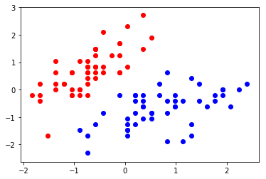
迭代次数越多很显然算法性能就越低，解决这个问题的令一个办法是数据归一化，使用 preprocessing 模块提供的 scale 方法将数据移到靠近中心的位置，让其符合正态分布，可以看出不用增加迭代次数算法也可以很快收敛：

from sklearn.svm import LinearSVC
from sklearn import preprocessing

X_scaled = preprocessing.scale(X)
svc = LinearSVC(C=1e9)
svc.fit(X_scaled, y)
results = svc.predict(preprocessing.scale([[6,2], [4, 3]]))
print(results)

plt.scatter(X_scaled[y == 0, 0], X_scaled[y == 0, 1], color='red')
plt.scatter(X_scaled[y == 1, 0], X_scaled[y == 1, 1], color='blue')
plt.show()

运行结果

[1 0]

运行结果

Notebook 运行结果

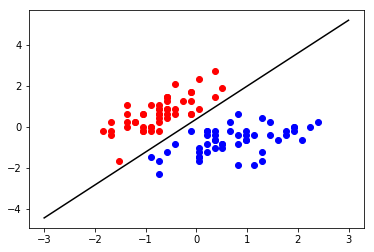
最后我们在图中画出划分超平面，也就是决策边界，决策边界为一条直线：

w_1x + w_2y + b = 0

这里的 $w$ 为特征系数，可以通过 svc.coef_ 取得， $b$ 为截距，可以通过 intercept_ 取得：

print('w = ', svc.coef_)
print('b = ', svc.intercept_)

运行结果

w =  [[ 4.03244052 -2.50699934]]
b =  [0.92733476]

从而得到直线方程：

y = -\frac{w_1x+b}{w_2}

def plot_svc_decision_boundary(model):
    w = model.coef_[0]
    b = model.intercept_[0]
    x = np.linspace(-3, 3, 200)
    y = - (w[0]*x+b) / w[1]
    plt.plot(x, y, color='black')

plot_svc_decision_boundary(svc)
plt.scatter(X_scaled[y == 0, 0], X_scaled[y == 0, 1], color='red')
plt.scatter(X_scaled[y == 1, 0], X_scaled[y == 1, 1], color='blue')
plt.show()

运行结果

Notebook 运行结果